本文脉络：首先回顾一下之前对贝叶斯神经网络的介绍，然后简述如何在贝叶斯神经网络进行反向传播。

回顾

之前讲到。普通的神经网络具有如下缺陷：

容易过拟合
无法表达不确定性

所以为了解决普通神经网络的以上缺陷，学者将贝叶斯引入到了神经网络中来，通过神经网络中权重的不确定性来使神经网络得以表达不确定性。

具体的做法就是，贝叶斯神经网络中的权重不再是一个固定的值，而是一个完整的分布。

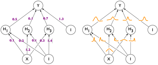
那我们应该如何求解贝叶斯神经网络中的参数呢？反向传播对于贝叶斯神经网络还适用吗？

我们先来回顾一下普通神经网络中参数的求解。

我们将一个神经网络视为这样一个概率模型：

$$ P(y\mid x,w) $$

在给定一个输入$x \in R$ 的情况下，神经网络会使用一组参数 $w$ 为每个可能的输出分配一个概率 $y\in Y$。

对于分类模型：$P(y\mid x,w)$ 为多分类分布，对应的是交叉熵损失
对于回归模型：$P(y\mid x, w)$为高斯分布，对应的是均方差损失

模型中的参数通过极大似然估计（MLE）求解：

$$ \begin{equation*}\begin{aligned}\mathbf{w}^{\mathrm{MLE}} &=\arg \max {\mathbf{w}} \log P(\mathcal{D} \mid \mathbf{w}) \&=\arg \max {\mathbf{w}} \sum{i} \log P\left(\mathbf{y}{i} \mid \mathbf{x}_{i}, \mathbf{w}\right)\end{aligned}\end{equation*} $$

如果引入正则化后，则对应的极大后验估计：

$$ \begin{equation*}\begin{aligned}\mathbf{w}^{\text {MAP }} &=\arg \max _{\mathbf{w}} \log P(\mathbf{w} \mid \mathcal{D}) \&=\arg \max _{\mathbf{w}} \log P(\mathcal{D} \mid \mathbf{w})+\log P(\mathbf{w})\end{aligned}\end{equation*} $$

且在极大后验估计中，如果先验 $P(w)$ 为高斯分布，那么对应的是$L2$正则化，如果先验 $P(w)$ 为拉普拉斯分布，那么对应的是$L1$正则化。

具体参数通过梯度下降来求解。

贝叶斯神经网络中的变分近似

贝叶斯神经网络

贝叶斯神经网络中的参数均为一个个随机变量，我们想要的是这个随机变量的完整的分布。根据贝叶斯公式：

$$ \begin{equation*}P(W \mid D)=\frac{P(W) P(D \mid W)}{P(D)} = \frac {P(W) P(D \mid W)}{{\large \int} P(W) P(D \mid W) dW}\end{equation*} $$

现在想算出后验$P(W\mid D)$,我们做如下尝试：

☹️计算后验解析解。由全概率公式可知，分母 $P(D)$ 为在 $w$ 的取值空间上进行积分，我们知道神经网络的单个权重的取值空间为实数集，而这些权重一起构成的空间将相当复杂，所以想要通过积分计算 $P(D)$ 解析解，基本是不可能的。
☹️通过采样计算 $P(D)$ 。通过蒙特卡洛采样来计算分母 $P(D)$ 的积分。然而着要求从一个相当高的维度分布中采样。理论上可行，但实践中太过于消耗时间了。
😄变分推断。**采用一些简单的分布去近似后验分布 **$P(W\mid D)$

变分引入

普通神经网络中，每个权重都是一个固定值，为贝叶斯神经网络中，权重为一个分布。现在我们用高斯分布去近似每个权重的分布。

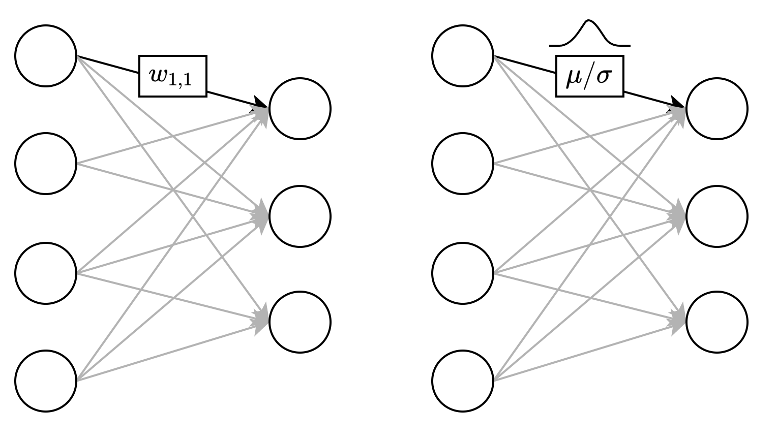
对于权重 $w_i$ 的分布, 我们用高斯分布 $\mathcal N(\mu_i, \sigma_i)$ 来近似，形式化表达如下：

$$ w_i \approx \mathcal N(\mu_i, \sigma_i) $$

将新引进来的所有参数表示为 $\theta$：

$$ \theta = (\mu, \sigma) $$

此时，我们就定义以下的变分分布，该变分分布包括了神经网络中所有权重的分布：

$$ q(w \vert \theta) $$

此时我们的目的就很清晰了，选择最佳的 $\theta$，使得我们构造出来的变分分布与目标后验分布最接近。

$变分分布q(w \mid \theta) 与目标后验分布P(W\mid D)$

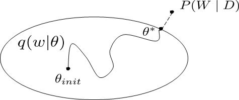
那么就有一个问题，应该如何衡量这两个分布之间的差异呢？在这里，选择采用KL散度度量量分布之间的差异：

$$ \begin{equation*}\text{KL}[q(w \mid \theta) | P(w \mid \mathcal{D})]\end{equation*} $$

变分学习

这个时候我们的问题已经很清晰了，找到一组合适的参数\theta，使得变分分布 $q(w\mid \theta)$ 与后验分布 $P(W\mid D)$ 的 $\text{KL}$ 散度最小。形式化表达如下：

$$ \begin{equation*}\begin{aligned}\theta^{} &=\arg \min _{w} K L[q(w \mid \theta) | P(w \mid \mathcal{D})] \&=\arg \min _{w} \int q(w \mid \theta) \log \frac{q(w \mid \theta)}{P(w) P(\mathcal{D} \mid w)} d w \&=\arg \min {\theta} K L[q(w \mid \theta) | P(w)]-\mathbb{E}{q(w \mid \theta)}[\log P(\mathcal{D} \mid w)]\end{aligned}\end{equation} $$

$\text{KL}$ 散度即可以看作是我们普通神经网络中的损失函数，为了简单，我们将其用 $\mathcal{F}(\mathcal{D}, \theta)$ 表示：

$$ \begin{equation*}\begin{split}\mathcal{F}(\mathcal{D}, \theta)&=K L[q(w \mid \theta) | P(w)]-\mathbb{E}{q(w \mid \theta)}[\log P(\mathcal{D} \mid w)]\&= \mathbb{E}{q(w \mid \theta)}[{\log q(w \mid \theta)-P(w) -P(\mathcal{D} \mid w)}]\end{split}\end{equation*} $$

精确的计算这个损失函数的最小化是相当困难的，实际上，我们采用梯度下降来求解。

但是这就有哟个问题，我们该如何对一个函数的期望求梯度呢？

论文中提出这样一个命题：

Proposition 1. Let 𝜖 be a random variable having a probability density given by 𝑞(𝜖) and let 𝑤 = 𝑡(𝜃,𝜖) where 𝑡(𝜃,𝜖) is a deterministic function. Suppose further that the marginal probability density of 𝑤, 𝑞(𝑤∣𝜃), is such that 𝑞(𝜖)𝑑𝜖= 𝑞(𝑤∣𝜃)𝑑𝑤. Then for a function 𝑓 with derivatives in 𝑤: $$ \begin{equation*}\frac{\partial}{\partial \theta} \mathbb{E}{q(w \mid \theta)}[f(w, \theta)]=\mathbb{E}{q(\epsilon)}\left[\frac{\partial f(w, \theta)}{\partial w} \frac{\partial w}{\partial \theta}+\frac{\partial f(w, \theta)}{\partial \theta}\right]\end{equation*} $$

简单来说，就是在满足一定的条件下，期望的导数可以被表示为导数的期望。恰好，我们的目标函数$\mathcal{F}(\mathcal{D}, \theta)$ 是满足这样条件的。所以我们就可以直接对 $\mathcal{F}(\mathcal{D}, \theta)$ 求梯度，然后再对梯度求期望。其中，对梯度求期望可以通过多次采样求平均来实现。

所以现在我们的目标函数转化为 $f(w, \theta)$:

$$ f(w, \theta)=\log q(w \mid \theta)-\log P(w) P(\mathcal{D} \mid w) $$

我们可以通过求$\frac{\partial }{\partial \theta} f(w,\theta)$ 的多次采样的均值来估计 $\frac{\partial }{\partial \theta} \mathcal{F}(\mathcal{D}, \theta)$

至此，优化问题就转化为了

$$ \begin{equation*}\begin{aligned}\theta^{} &=\arg \min _{w} \log q(w \mid \theta)-\log P(w) P(\mathcal{D} \mid w)\end{aligned}\end{equation} $$

我们通过梯度下降来求解 $\theta ^*$:

采样得到 $w$, $w \sim q(w \mid \theta), \theta=(\mu, \sigma).$ 采样的过程不可导，所以这里采用了一个重参数化的技巧，另 $$ \begin{equation*}\mathbf{w}=\mu+\log (1+\exp (\rho)) \circ \epsilon\end{equation*} $$ 此时，对 $w$ 采样就转化为了对 $\epsilon \sim \mathcal{N}(0,1)$ 采样，同时参数转化为了 $\theta = (\mu, \rho)$
计算损失函数值 $f(w, \theta)$
1. 计算似然 $$ \begin{equation*}P(D|w) = \sum_i^N \log(P(y_i|w,x_i))\end{equation*} $$
2. 计算损失值： $$ f(w, \theta)=\log q(w \mid \theta)-\log P(w) P(\mathcal{D} \mid w) $$
计算梯度： $$ \begin{equation*}\begin{aligned}\Delta_{\mu}&=\frac{\partial f(\mathrm{w}, \theta)}{\partial \mathrm{w}}+\frac{\partial f(\mathrm{w}, \theta)}{\partial \mu}\\Delta_{\rho}&=\frac{\partial f(\mathbf{w}, \theta)}{\partial \mathbf{w}} \frac{\epsilon}{1+\exp (-\rho)}+\frac{\partial f(\mathbf{w}, \theta)}{\partial \rho} \end{aligned}\end{equation*} $$
更新参数 $$ \begin{equation*}\begin{aligned}&\mu \leftarrow \mu-\alpha \Delta_{\mu} \&\rho \leftarrow \rho-\alpha \Delta_{\rho}\end{aligned}\end{equation*} $$

小结

贝叶斯神经网络中的参数W为随机变量，我们想要求得这个随机变量的完整分布，然后在前向传播的时候，通过采样得到的权重值具有不确定度，进而使得整个神经网络可以表达不确定度。

参数W完整的分布称为后验分布，由贝叶斯公式：

$$ \begin{equation*}P(W \mid D)=\frac{P(W) P(D \mid W)}{P(D)}\end{equation*} $$

可知，想要计算后验的解析解是异常困难的，所以这里我们通过一些简单的分布来近似这个后验分布，这个过程称之为变分近似，这些个简单的分布称为变分分布。

我们通过\text{KL} 散度来度量变分分布于后验分布的差异，所以有了如下的优化问题：

$$ \begin{equation*}\theta^{}=\underset{\theta}{\operatorname{argmin}} \mathrm{KL}[q(w \mid \theta) | P(w \mid \mathcal{D})]\end{equation} $$

在解这个优化问题的过程中，使用了一个命题和一个重参数化的技巧：

命题：在满足一定的条件下，期望的导数可以表示为导数的期望 $$ \begin{equation*}\frac{\partial}{\partial \theta} \mathbb{E}{q(w \mid \theta)}[f(w, \theta)]=\mathbb{E}{q(\epsilon)}\left[\frac{\partial f(w, \theta)}{\partial w} \frac{\partial w}{\partial \theta}+\frac{\partial f(w, \theta)}{\partial \theta}\right]\end{equation*} $$
重参数技巧：将对 $w$ 的采用转化为了对 $\epsilon$ 的采样： $$ \mathbf{w}=\mu+\log (1+\exp (\rho)) \circ \epsilon $$

最后，优化问题转化为了：

$$ \begin{equation*}\begin{aligned}\theta^{} &=\arg \min _{w} \log q(w \mid \theta)-\log P(w) P(\mathcal{D} \mid w)\end{aligned}\end{equation} $$

最后

最后我们看一下该如何在Pytorch中编写这样一个贝叶斯神经网络全连接层。

首先来看一下Pytorch中的普通神经网络全连接层：

class Linear(nn.Module):
    def __init__(self, in_features, out_features):
        super(Linear, self).__init__()
        
        self.in_features = in_features
        self.out_features = out_features
        
				# 定义两个参数 
        self.w = nn.Parameter(torch.empty((out_features, in_features)))  
        self.b = nn.Parameter(torch.empty((out_features)))
                           
        self.w.data.normal_(mean = 0, std = 0.01)
        self.b.data.fill_(0.0)
                           
    def forward(self, input):
        return torch.matmul(input, self.w.T) + self.b

那如果要实现贝叶斯神经网络全连接层，就需要这么写：

class BayesLinear(nn.Module):
    def __init__(self, in_feature, out_feature, prior_var=1.0):
        super(BayesLinear,self).__init__()
        self.in_feature = in_feature
        self.out_feature = out_feature
        
        # 权重的分布
        self.w_mu = nn.Parameter(torch.zeros(self.out_feature, self.in_feature))
        self.w_rho = nn.Parameter(torch.zeros(self.out_feature, self.in_feature))
        
        # 偏置的分布
        self.b_mu = nn.Parameter(torch.zeros(self.out_feature))
        self.b_rho = nn.Parameter(torch.zeros(self.out_feature))
        
        # 权重 和偏置
        self.w = None
        self.b = None
        
        # 初始化先验分布
        self.prior = torch.distributions.Normal(0, prior_var)
        
    def forward(self, input):
        # 采样得到 权重和偏执
        # 这里 epsion shape 和mu.shape 是一样的，是一对一的
        w_epsilon = torch.distributions.Normal(0, 1).sample(self.w_mu.shape)
        self.w = self.w_mu + torch.log(1+torch.exp(self.w_rho)) * w_epsilon
        
        b_epsilon = Normal(0,1).sample(self.b_mu.shape)
        self.b = self.b_mu + torch.log(1+torch.exp(self.b_rho)) * b_epsilon
        
        # 计算先验概率 
        w_log_prior = self.prior.log_prob(self.w)
        b_log_prior = self.prior.log_prob(self.b)
        self.log_prior = torch.sum(w_log_prior) + torch.sum(b_log_prior)
        
        # 计算变分分布
        self.w_post = torch.distributions.Normal(self.w_mu.data, torch.log(1+torch.exp(self.w_rho)))
        self.b_post = torch.distributions.Normal(self.b_mu.data, torch.log(1+torch.exp(self.b_rho)))
        # 计算变分后验概率
        self.log_post = self.w_post.log_prob(self.w).sum() + self.b_post.log_prob(self.b).sum()
        
        return torch.matmul(input, self.w.T) + self.b

可见，贝叶斯神经网络全连接层中的参数数量为普通神经网络参数数量的二倍。

参考

论文：Weight Uncertainty in Neural Networks, Blundell et al

Blog： Weight Uncertainty in Neural Networks Tutorial

视频：贝叶斯神经网络

贝叶斯神经网络变分近似

回顾

贝叶斯神经网络中的变分近似

贝叶斯神经网络

变分引入

变分学习

小结

最后

参考